Data cleaning with dplyr and tidyr: Handling missing values, data reshaping, and filtering.
Exploratory Data Analysis (EDA): Summary statistics, data visualization, and feature engineering.
Hands-on exercises to perform data cleaning and EDA on a dataset collected during Day 1.
8.0.2 Outcome
Participants will be able to clean data and conduct exploratory analyses to derive insights.
8.1 Introduction to Data Cleaning
Data cleaning is an essential step in preparing your dataset for analysis. The dplyr and tidyr packages in R provide powerful tools for transforming and tidying data.
8.1.1 Example: Handling Missing Values
Show the code
library(dplyr)
Attaching package: 'dplyr'
The following objects are masked from 'package:stats':

    filter, lag
The following objects are masked from 'package:base':

    intersect, setdiff, setequal, union
Show the code
# Sample dataset with missing valuesdata <-tibble(id =1:5,value =c(10, NA, 30, NA, 50))# Remove rows with missing valuesclean_data <- data %>%filter(!is.na(value))# Display cleaned dataclean_data
# A tibble: 3 × 2
     id value
  <int> <dbl>
1     1    10
2     3    30
3     5    50
8.1.2 Example: Reshaping Data
Show the code
library(tidyr)# Sample dataset for reshapingwide_data <-tibble(id =1:3,score_1 =c(80, 85, 90),score_2 =c(70, 75, 80))# Convert from wide to long formatlong_data <- wide_data %>%pivot_longer(cols =starts_with("score"), names_to ="test", values_to ="score")# Display reshaped datalong_data
8.2 Introduction to Exploratory Data Analysis (EDA)
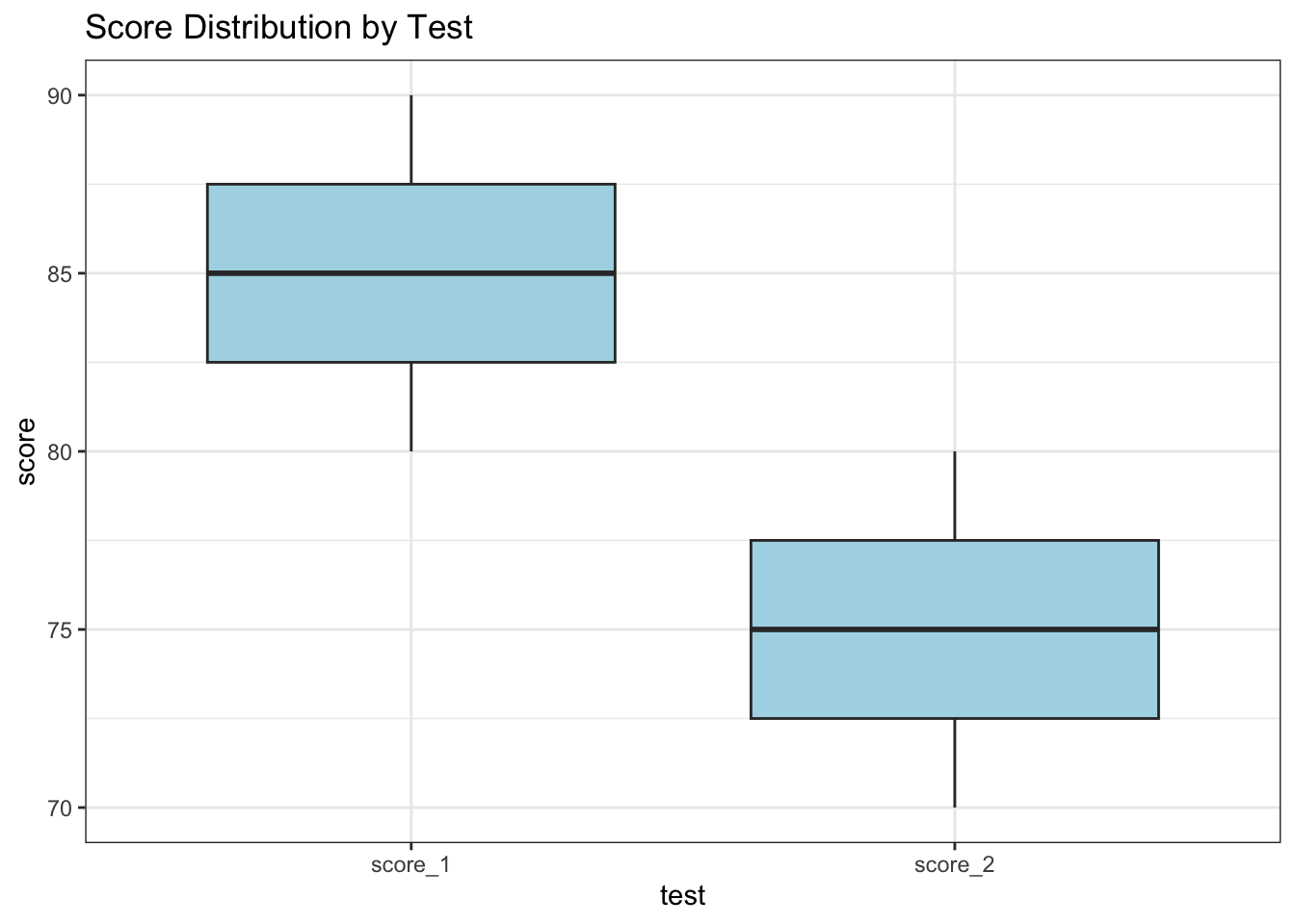
EDA involves summarizing the main characteristics of a dataset often using visual methods. It helps in understanding the patterns, anomalies, and relationships within the data.
library(ggplot2)# Visualize the distribution of scoresggplot(long_data, aes(x = test, y = score)) +geom_boxplot(fill ="lightblue") +labs(title ="Score Distribution by Test") +theme_bw()
8.3 Hands-On Exercise
8.3.1 Exercise 1: Clean a Dataset
Use a dataset collected during Day 1.
Identify and handle missing values using dplyr.
Show the code
# Example code structure for cleaning a datasetdataset <-tibble(id =c(1, 2, NA, 4),value =c(10, NA, 30, NA))cleaned_dataset <- dataset %>%drop_na() # Remove rows with any missing valuescleaned_dataset
# A tibble: 1 × 2
     id value
  <dbl> <dbl>
1     1    10
8.3.2 Exercise 2: Perform EDA
Generate summary statistics for your cleaned dataset.
Create visualizations to explore relationships in the data using ggplot2.
Show the code
# Example code structure for EDAeda_summary <- cleaned_dataset %>%summarise(mean_value =mean(value))ggplot(cleaned_dataset, aes(x = id, y = value)) +geom_point() +labs(title ="Value by ID") +theme_bw()
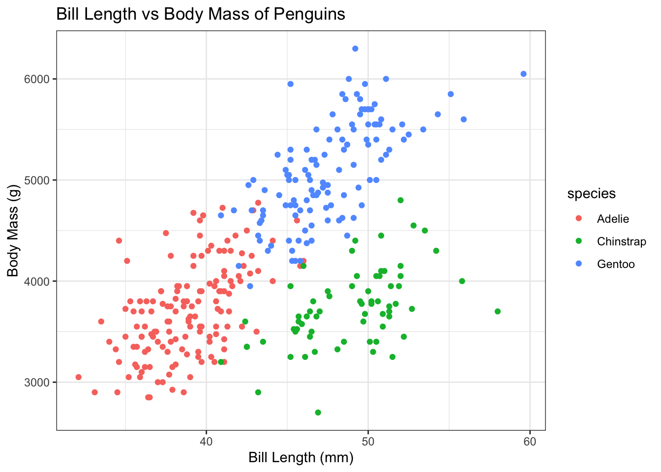
Description: This dataset contains information about three species of penguins (Adélie, Gentoo, and Chinstrap) from the Palmer Archipelago in Antarctica. It includes variables such as species, island, bill length, bill depth, flipper length, body mass, and sex.
Exercises: - Data Cleaning: Check for missing values and handle them appropriately. For example, decide whether to impute missing values or remove rows with missing data. - Exploratory Analysis: Create visualizations to compare the physical characteristics (e.g., bill length vs. body mass) among the three species of penguins. - Statistical Analysis: Perform a t-test to determine if there are significant differences in body mass between the species.
Show the code
# Load necessary librarieslibrary(palmerpenguins)library(ggplot2)library(dplyr)# View the datasethead(penguins)
# A tibble: 6 × 8
  species island    bill_length_mm bill_depth_mm flipper_length_mm body_mass_g
  <fct>   <fct>              <dbl>         <dbl>             <int>       <int>
1 Adelie  Torgersen           39.1          18.7               181        3750
2 Adelie  Torgersen           39.5          17.4               186        3800
3 Adelie  Torgersen           40.3          18                 195        3250
4 Adelie  Torgersen           NA            NA                  NA          NA
5 Adelie  Torgersen           36.7          19.3               193        3450
6 Adelie  Torgersen           39.3          20.6               190        3650
# ℹ 2 more variables: sex <fct>, year <int>
Show the code
# Data cleaning: Remove rows with NA valuescleaned_penguins <-na.omit(penguins)# Exploratory analysis: Visualize bill length vs. body mass by speciesggplot(cleaned_penguins, aes(x = bill_length_mm, y = body_mass_g, color = species)) +geom_point() +labs(title ="Bill Length vs Body Mass of Penguins",x ="Bill Length (mm)",y ="Body Mass (g)") +theme_bw()
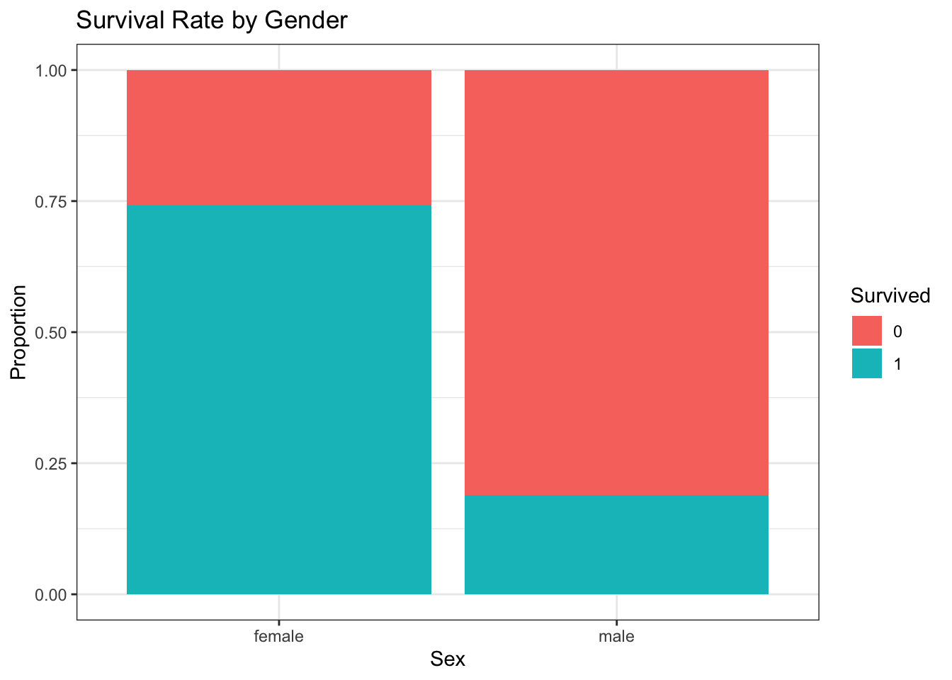
Description: This famous dataset contains information about the passengers on the Titanic, including their survival status, age, class, sex, fare paid, and more.
Exercises: - Data Cleaning: Identify and handle missing values in the dataset. For example, impute missing ages using the median or mean age based on passenger class. - Exploratory Analysis: Analyze survival rates based on different factors such as gender and passenger class. Create visualizations to illustrate your findings. - Feature Engineering: Create a new feature that categorizes passengers into age groups (e.g., child, adult) and analyze survival rates based on this new feature.
Show the code
# Load necessary librarieslibrary(tidyverse)
── Attaching core tidyverse packages ──────────────────────── tidyverse 2.0.0 ──
✔ forcats   1.0.0     ✔ readr     2.1.5
✔ lubridate 1.9.3     ✔ stringr   1.5.1
✔ purrr     1.0.2     ✔ tibble    3.2.1
── Conflicts ────────────────────────────────────────── tidyverse_conflicts() ──
✖ dplyr::filter() masks stats::filter()
✖ dplyr::lag()    masks stats::lag()
ℹ Use the conflicted package (<http://conflicted.r-lib.org/>) to force all conflicts to become errors
Show the code
# Load Titanic datasettitanic_data <-read.csv("https://raw.githubusercontent.com/datasciencedojo/datasets/refs/heads/master/titanic.csv")# Data cleaning: Impute missing ages with median agetitanic_data$Age[is.na(titanic_data$Age)] <-median(titanic_data$Age, na.rm =TRUE)# Exploratory analysis: Survival rate by genderggplot(titanic_data, aes(x = Sex, fill =factor(Survived))) +geom_bar(position ="fill") +labs(title ="Survival Rate by Gender",y ="Proportion",fill ="Survived") +theme_bw()
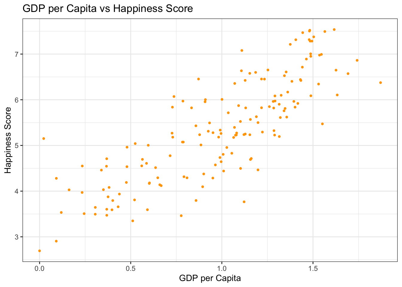
Description: This dataset includes happiness scores for countries around the world based on various factors such as GDP per capita, social support, life expectancy, freedom to make life choices, generosity, and perceptions of corruption.
Exercises: - Data Cleaning: Check for any inconsistencies or missing values in the dataset. Clean the data as necessary. - Exploratory Analysis: Analyze the relationship between GDP per capita and happiness scores using scatter plots. Use regression analysis to model this relationship. - Comparative Analysis: Compare happiness scores across different regions or continents using boxplots.
Show the code
happiness_data <-read.csv("https://raw.githubusercontent.com/datageneration/nchu/refs/heads/main/datascience/data/2017.csv")# Data cleaning: Check for NA valuessummary(happiness_data)
   Country          Happiness.Rank  Happiness.Score  Whisker.high
 Length:155         Min.   :  1.0   Min.   :2.693   Min.   :2.865
 Class :character   1st Qu.: 39.5   1st Qu.:4.505   1st Qu.:4.608
 Mode  :character   Median : 78.0   Median :5.279   Median :5.370
                    Mean   : 78.0   Mean   :5.354   Mean   :5.452
                    3rd Qu.:116.5   3rd Qu.:6.101   3rd Qu.:6.195
                    Max.   :155.0   Max.   :7.537   Max.   :7.622
  Whisker.low    GDP.per.capita       Family      Health..Life.Expectancy.
 Min.   :2.521   Min.   :0.0000   Min.   :0.000   Min.   :0.0000
 1st Qu.:4.375   1st Qu.:0.6634   1st Qu.:1.043   1st Qu.:0.3699
 Median :5.193   Median :1.0646   Median :1.254   Median :0.6060
 Mean   :5.256   Mean   :0.9847   Mean   :1.189   Mean   :0.5513
 3rd Qu.:6.007   3rd Qu.:1.3180   3rd Qu.:1.414   3rd Qu.:0.7230
 Max.   :7.480   Max.   :1.8708   Max.   :1.611   Max.   :0.9495
    Freedom         Generosity     Trust..Government.Corruption.
 Min.   :0.0000   Min.   :0.0000   Min.   :0.00000
 1st Qu.:0.3037   1st Qu.:0.1541   1st Qu.:0.05727
 Median :0.4375   Median :0.2315   Median :0.08985
 Mean   :0.4088   Mean   :0.2469   Mean   :0.12312
 3rd Qu.:0.5166   3rd Qu.:0.3238   3rd Qu.:0.15330
 Max.   :0.6582   Max.   :0.8381   Max.   :0.46431
 Dystopia.Residual
 Min.   :0.3779
 1st Qu.:1.5913
 Median :1.8329
 Mean   :1.8502
 3rd Qu.:2.1447
 Max.   :3.1175
Show the code
# Exploratory analysis: Scatter plot of GDP vs Happiness Scoreggplot(happiness_data, aes(x = GDP.per.capita, y = Happiness.Score)) +geom_point(pch=20, color ="orange") +labs(title ="GDP per Capita vs Happiness Score",x ="GDP per Capita",y ="Happiness Score") +theme_bw()
By following these examples and exercises, participants will gain practical experience in data cleaning and exploratory data analysis using R. This session will enhance their ability to derive meaningful insights from raw datasets.
8.3.4 Recap
Data Cleaning: Introduces techniques for handling missing values and reshaping data using dplyr and tidyr.
Exploratory Data Analysis: Demonstrates how to calculate summary statistics and visualize data patterns with ggplot2.
Exercises: Provides hands-on practice for participants to apply these techniques on real datasets.
Source Code
# Chapter 7: Data Management and Exploratory Data Analysis (EDA)### Key Topics- Data cleaning with `dplyr` and `tidyr`: Handling missing values, data reshaping, and filtering.- Exploratory Data Analysis (EDA): Summary statistics, data visualization, and feature engineering.- Hands-on exercises to perform data cleaning and EDA on a dataset collected during Day 1.### OutcomeParticipants will be able to clean data and conduct exploratory analyses to derive insights.## Introduction to Data CleaningData cleaning is an essential step in preparing your dataset for analysis. The `dplyr` and `tidyr` packages in R provide powerful tools for transforming and tidying data.### Example: Handling Missing Values```{r}library(dplyr)# Sample dataset with missing valuesdata <-tibble(id =1:5,value =c(10, NA, 30, NA, 50))# Remove rows with missing valuesclean_data <- data %>%filter(!is.na(value))# Display cleaned dataclean_data```### Example: Reshaping Data```{r}library(tidyr)# Sample dataset for reshapingwide_data <-tibble(id =1:3,score_1 =c(80, 85, 90),score_2 =c(70, 75, 80))# Convert from wide to long formatlong_data <- wide_data %>%pivot_longer(cols =starts_with("score"), names_to ="test", values_to ="score")# Display reshaped datalong_data```## Introduction to Exploratory Data Analysis (EDA)EDA involves summarizing the main characteristics of a dataset often using visual methods. It helps in understanding the patterns, anomalies, and relationships within the data.### Example: Summary Statistics```{r}# Calculate summary statisticssummary_stats <- clean_data %>%summarise(mean_value =mean(value),median_value =median(value),sd_value =sd(value) )# Display summary statisticssummary_stats```### Example: Data Visualization with ggplot2```{r}library(ggplot2)# Visualize the distribution of scoresggplot(long_data, aes(x = test, y = score)) +geom_boxplot(fill ="lightblue") +labs(title ="Score Distribution by Test") +theme_bw()```## Hands-On Exercise### Exercise 1: Clean a Dataset1. Use a dataset collected during Day 1.2. Identify and handle missing values using `dplyr`.```{r}# Example code structure for cleaning a datasetdataset <-tibble(id =c(1, 2, NA, 4),value =c(10, NA, 30, NA))cleaned_dataset <- dataset %>%drop_na() # Remove rows with any missing valuescleaned_dataset```### Exercise 2: Perform EDA1. Generate summary statistics for your cleaned dataset.2. Create visualizations to explore relationships in the data using `ggplot2`.```{r}# Example code structure for EDAeda_summary <- cleaned_dataset %>%summarise(mean_value =mean(value))ggplot(cleaned_dataset, aes(x = id, y = value)) +geom_point() +labs(title ="Value by ID") +theme_bw()```### Exercises with Real Datasets#### 1. **Penguins Dataset****Source:** [Palmer Penguins Dataset](https://allisonhorst.github.io/palmerpenguins/)**Description:** This dataset contains information about three species of penguins (Adélie, Gentoo, and Chinstrap) from the Palmer Archipelago in Antarctica. It includes variables such as species, island, bill length, bill depth, flipper length, body mass, and sex.**Exercises:** - **Data Cleaning:** Check for missing values and handle them appropriately. For example, decide whether to impute missing values or remove rows with missing data. - **Exploratory Analysis:** Create visualizations to compare the physical characteristics (e.g., bill length vs. body mass) among the three species of penguins. - **Statistical Analysis:** Perform a t-test to determine if there are significant differences in body mass between the species.``` {r}# Load necessary librarieslibrary(palmerpenguins)library(ggplot2)library(dplyr)# View the datasethead(penguins)# Data cleaning: Remove rows with NA valuescleaned_penguins <- na.omit(penguins)# Exploratory analysis: Visualize bill length vs. body mass by speciesggplot(cleaned_penguins, aes(x = bill_length_mm, y = body_mass_g, color = species)) + geom_point() + labs(title = "Bill Length vs Body Mass of Penguins", x = "Bill Length (mm)", y = "Body Mass (g)") + theme_bw()```#### 2. **Titanic Dataset****Source:** [Kaggle Titanic Dataset](https://www.kaggle.com/c/titanic/data)**Description:** This famous dataset contains information about the passengers on the Titanic, including their survival status, age, class, sex, fare paid, and more.**Exercises:** - **Data Cleaning:** Identify and handle missing values in the dataset. For example, impute missing ages using the median or mean age based on passenger class. - **Exploratory Analysis:** Analyze survival rates based on different factors such as gender and passenger class. Create visualizations to illustrate your findings. - **Feature Engineering:** Create a new feature that categorizes passengers into age groups (e.g., child, adult) and analyze survival rates based on this new feature.```{r}# Load necessary librarieslibrary(tidyverse)# Load Titanic datasettitanic_data <-read.csv("https://raw.githubusercontent.com/datasciencedojo/datasets/refs/heads/master/titanic.csv")# Data cleaning: Impute missing ages with median agetitanic_data$Age[is.na(titanic_data$Age)] <-median(titanic_data$Age, na.rm =TRUE)# Exploratory analysis: Survival rate by genderggplot(titanic_data, aes(x = Sex, fill =factor(Survived))) +geom_bar(position ="fill") +labs(title ="Survival Rate by Gender",y ="Proportion",fill ="Survived") +theme_bw()```#### 3. **World Happiness Report****Source:** [World Happiness Report Dataset](https://www.kaggle.com/datasets/unsdsn/world-happiness)**Description:** This dataset includes happiness scores for countries around the world based on various factors such as GDP per capita, social support, life expectancy, freedom to make life choices, generosity, and perceptions of corruption.**Exercises:** - **Data Cleaning:** Check for any inconsistencies or missing values in the dataset. Clean the data as necessary. - **Exploratory Analysis:** Analyze the relationship between GDP per capita and happiness scores using scatter plots. Use regression analysis to model this relationship. - **Comparative Analysis:** Compare happiness scores across different regions or continents using boxplots.``` {r}happiness_data <- read.csv("https://raw.githubusercontent.com/datageneration/nchu/refs/heads/main/datascience/data/2017.csv")# Data cleaning: Check for NA valuessummary(happiness_data)# Exploratory analysis: Scatter plot of GDP vs Happiness Scoreggplot(happiness_data, aes(x = GDP.per.capita, y = Happiness.Score)) + geom_point(pch=20, color = "orange") + labs(title = "GDP per Capita vs Happiness Score", x = "GDP per Capita", y = "Happiness Score") + theme_bw()```By following these examples and exercises, participants will gain practical experience in data cleaning and exploratory data analysis using R. This session will enhance their ability to derive meaningful insights from raw datasets. ### Recap- **Data Cleaning:** Introduces techniques for handling missing values and reshaping data using `dplyr` and `tidyr`.- **Exploratory Data Analysis:** Demonstrates how to calculate summary statistics and visualize data patterns with `ggplot2`.- **Exercises:** Provides hands-on practice for participants to apply these techniques on real datasets.