9 Chapter 8: Introduction to Machine Learning Models in R

9.0.1 Key Topics

Basics of machine learning models in R, focusing on regression and classification models.
Using R packages such as caret or tidymodels for training simple models.
Hands-on exercises to build a basic predictive model, evaluate its performance, and interpret the results.

9.0.2 Outcome

Participants will understand the fundamentals of machine learning models and build their own in R.

9.1 Introduction to Machine Learning Models

Machine learning involves using algorithms to identify patterns within data. In R, packages like caret and tidymodels simplify the process of training and evaluating machine learning models.

9.1.1 Example: Linear Regression with caret

Show the code

# install.packages("caret")
library(caret)

# Load dataset
data(mtcars)

# Split data into training and testing sets
set.seed(123)
trainIndex <- createDataPartition(mtcars$mpg, p = .8, 
                                  list = FALSE, 
                                  times = 1)
trainData <- mtcars[ trainIndex,]
testData  <- mtcars[-trainIndex,]

# Train a linear regression model
model <- train(mpg ~ ., data = trainData, method = "lm")

# Summary of the model
summary(model)


Call:
lm(formula = .outcome ~ ., data = dat)

Residuals:
    Min      1Q  Median      3Q     Max 
-3.2742 -1.3609 -0.2707  1.1921  4.9877 

Coefficients:
            Estimate Std. Error t value Pr(>|t|)
(Intercept) -2.81069   22.93545  -0.123    0.904
cyl          0.75593    1.21576   0.622    0.542
disp         0.01172    0.01674   0.700    0.494
hp          -0.01386    0.02197  -0.631    0.536
drat         2.24007    1.77251   1.264    0.223
wt          -2.73273    1.87954  -1.454    0.164
qsec         0.53957    0.71812   0.751    0.463
vs           1.21640    2.02623   0.600    0.556
am           1.73662    2.08358   0.833    0.416
gear         2.95127    1.88459   1.566    0.136
carb        -1.19910    0.98232  -1.221    0.239

Residual standard error: 2.431 on 17 degrees of freedom
Multiple R-squared:  0.8861,    Adjusted R-squared:  0.8191 
F-statistic: 13.23 on 10 and 17 DF,  p-value: 3.719e-06

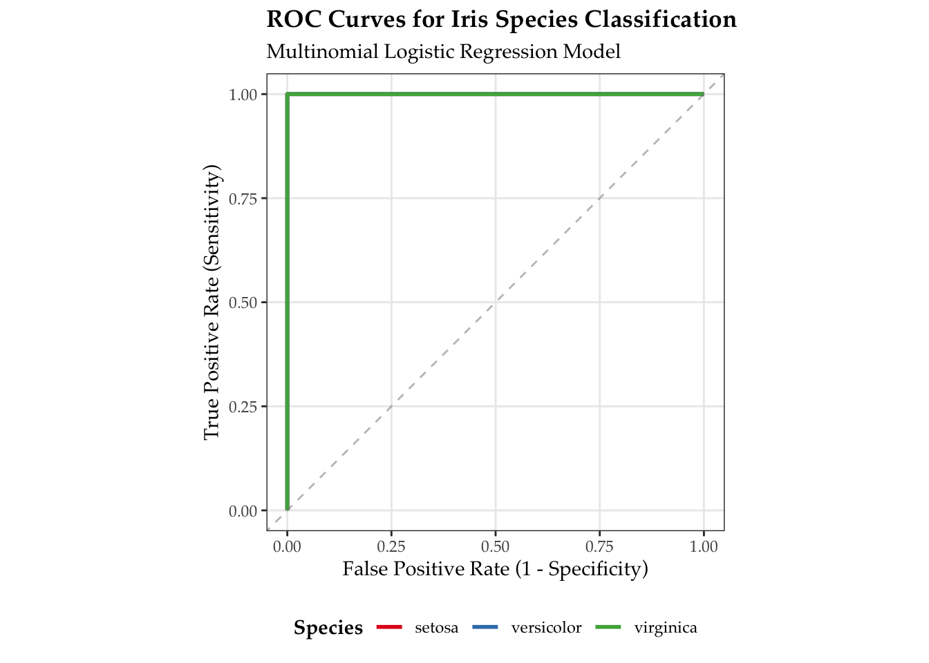
9.1.2 Example: Classification with tidymodels

Show the code

library(tidymodels)
library(ggplot2)

# Split the data
set.seed(123)
iris_split <- initial_split(iris, prop = 0.8)
iris_train <- training(iris_split)
iris_test <- testing(iris_split)


# Fit model
multi_log_reg_model <- multinom_reg() %>% 
  set_engine("nnet") %>% 
  fit(Species ~ ., data = iris_train)


# Generate predictions with proper format
predictions <- predict(multi_log_reg_model, iris_test, type = "prob") %>%
  bind_cols(iris_test %>% select(Species))

# Calculate ROC curve data
roc_data <- roc_curve(
  predictions,
  truth = Species,
  .pred_setosa, .pred_versicolor, .pred_virginica
)

# Plot the ROC curves
roc_plot <- ggplot(roc_data, aes(x = 1 - specificity, y = sensitivity, color = .level)) +
  geom_path(linewidth = 1) +
  geom_abline(lty = 2, alpha = 0.5, color = "gray50", slope = 1, intercept = 0) +
  coord_equal() +
  labs(
    title = "ROC Curves for Iris Species Classification",
    subtitle = paste("Multinomial Logistic Regression Model"),
    x = "False Positive Rate (1 - Specificity)",
    y = "True Positive Rate (Sensitivity)",
    color = "Species"
  ) +
  scale_color_brewer(palette = "Set1") +
  theme_bw() +
  theme(
    text = element_text(family = "Palatino"),
    legend.position = "bottom",
    panel.grid.minor = element_blank(),
    plot.title = element_text(face = "bold"),
    legend.title = element_text(face = "bold")
  )

# Calculate and add the AUC values to the plot
auc_values <- roc_auc(
  predictions,
  truth = Species,
  .pred_setosa, .pred_versicolor, .pred_virginica
)

# Print AUC values and display the plot
print(auc_values)

# A tibble: 1 × 3
  .metric .estimator .estimate
  <chr>   <chr>          <dbl>
1 roc_auc hand_till          1

Show the code

print(roc_plot)

9.2 Hands-On Exercise

9.2.1 Exercise 1: Build a Predictive Model

Use the mtcars dataset.
Train a linear regression model to predict mpg using caret.

Show the code

# Example code structure for building a predictive model
model_mtcars <- train(mpg ~ ., data = trainData, method = "lm")

summary(model_mtcars)

9.2.2 Exercise 2: Evaluate Model Performance

Evaluate the model on test data.
Interpret the results and discuss potential improvements.

Show the code

# Predict on test data
predictions_mtcars <- predict(model_mtcars, newdata = testData)

# Calculate RMSE
rmse(predictions_mtcars, testData$mpg)

9.3 References

Kuhn, M., & Johnson, K. (2013). Applied Predictive Modeling. Springer.
Wickham, H., & Grolemund, G. (2016). R for Data Science. O’Reilly Media.
Max Kuhn’s caret package documentation.
Tidymodels website for comprehensive guides and tutorials.

By following these examples and exercises, participants will gain practical experience in building and evaluating machine learning models using R. This session will enhance their ability to apply predictive modeling techniques to real-world datasets. ```

9.3.1 Recap

Machine Learning Basics: Introduces regression and classification models using caret and tidymodels.
Examples: Provides code snippets for training linear regression and logistic regression models.
Exercises: Offers hands-on practice for building and evaluating predictive models.
References: Lists useful resources for further reading and exploration of machine learning concepts in R.

This chapter ensures participants understand both theoretical concepts and practical applications of machine learning in R.

# Chapter 8: Introduction to Machine Learning Models in R ### Key Topics - Basics of machine learning models in R, focusing on regression and classification models. - Using R packages such as `caret` or `tidymodels` for training simple models. - Hands-on exercises to build a basic predictive model, evaluate its performance, and interpret the results. ### Outcome Participants will understand the fundamentals of machine learning models and build their own in R. ## Introduction to Machine Learning Models Machine learning involves using algorithms to identify patterns within data. In R, packages like `caret` and `tidymodels` simplify the process of training and evaluating machine learning models. ### Example: Linear Regression with caret ```{r} #| message: false #| warning: false # install.packages("caret") library(caret) # Load dataset data(mtcars) # Split data into training and testing sets set.seed(123) trainIndex <- createDataPartition(mtcars$mpg, p = .8, list = FALSE, times = 1) trainData <- mtcars[ trainIndex,] testData <- mtcars[-trainIndex,] # Train a linear regression model model <- train(mpg ~ ., data = trainData, method = "lm") # Summary of the model summary(model) ``` ### Example: Classification with tidymodels ```{r} #| message: false #| warning: false library(tidymodels) library(ggplot2) # Split the data set.seed(123) iris_split <- initial_split(iris, prop = 0.8) iris_train <- training(iris_split) iris_test <- testing(iris_split) # Fit model multi_log_reg_model <- multinom_reg() %>% set_engine("nnet") %>% fit(Species ~ ., data = iris_train) # Generate predictions with proper format predictions <- predict(multi_log_reg_model, iris_test, type = "prob") %>% bind_cols(iris_test %>% select(Species)) # Calculate ROC curve data roc_data <- roc_curve( predictions, truth = Species, .pred_setosa, .pred_versicolor, .pred_virginica ) # Plot the ROC curves roc_plot <- ggplot(roc_data, aes(x = 1 - specificity, y = sensitivity, color = .level)) + geom_path(linewidth = 1) + geom_abline(lty = 2, alpha = 0.5, color = "gray50", slope = 1, intercept = 0) + coord_equal() + labs( title = "ROC Curves for Iris Species Classification", subtitle = paste("Multinomial Logistic Regression Model"), x = "False Positive Rate (1 - Specificity)", y = "True Positive Rate (Sensitivity)", color = "Species" ) + scale_color_brewer(palette = "Set1") + theme_bw() + theme( text = element_text(family = "Palatino"), legend.position = "bottom", panel.grid.minor = element_blank(), plot.title = element_text(face = "bold"), legend.title = element_text(face = "bold") ) # Calculate and add the AUC values to the plot auc_values <- roc_auc( predictions, truth = Species, .pred_setosa, .pred_versicolor, .pred_virginica ) # Print AUC values and display the plot print(auc_values) print(roc_plot) ``` ## Hands-On Exercise ### Exercise 1: Build a Predictive Model 1. Use the `mtcars` dataset. 2. Train a linear regression model to predict `mpg` using `caret`. ```{r eval=F} # Example code structure for building a predictive model model_mtcars <- train(mpg ~ ., data = trainData, method = "lm") summary(model_mtcars) ``` ### Exercise 2: Evaluate Model Performance 1. Evaluate the model on test data. 2. Interpret the results and discuss potential improvements. ```{r eval=F} # Predict on test data predictions_mtcars <- predict(model_mtcars, newdata = testData) # Calculate RMSE rmse(predictions_mtcars, testData$mpg) ``` ## References - Kuhn, M., & Johnson, K. (2013). *Applied Predictive Modeling*. Springer. - Wickham, H., & Grolemund, G. (2016). *R for Data Science*. O'Reilly Media. - Max Kuhn's [caret package documentation](https://topepo.github.io/caret/index.html). - [Tidymodels website](https://www.tidymodels.org/) for comprehensive guides and tutorials. By following these examples and exercises, participants will gain practical experience in building and evaluating machine learning models using R. This session will enhance their ability to apply predictive modeling techniques to real-world datasets. \`\`\` ### Recap - **Machine Learning Basics:** Introduces regression and classification models using `caret` and `tidymodels`. - **Examples:** Provides code snippets for training linear regression and logistic regression models. - **Exercises:** Offers hands-on practice for building and evaluating predictive models. - **References:** Lists useful resources for further reading and exploration of machine learning concepts in R. This chapter ensures participants understand both theoretical concepts and practical applications of machine learning in R.