Show the code
library(ggplot2)

# Basic scatter plot
ggplot(data = mtcars, aes(x = wt, y = mpg)) +
  geom_point(size = .8, col="firebrick") + xlab("Vehicle Weight") +
  ylab("Miles per Gallon (MPG)") +
  theme_bw()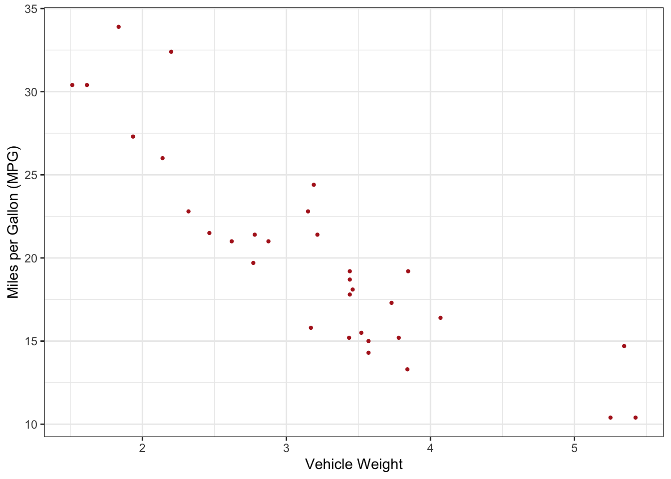
ggplot2 for data visualization.Plotly to add interactivity to charts.ggplot2 and enhance them with Plotly.Participants will create and embed interactive visualizations in Quarto using R.
ggplot2 is a powerful R package for creating static visualizations. It implements the Grammar of Graphics, allowing you to build complex plots from simple components.
Here is a simple example of creating a scatter plot using ggplot2:
library(ggplot2)
# Basic scatter plot
ggplot(data = mtcars, aes(x = wt, y = mpg)) +
geom_point(size = .8, col="firebrick") + xlab("Vehicle Weight") +
ylab("Miles per Gallon (MPG)") +
theme_bw()
You can customize the appearance of your plots by adjusting point size, shape, and color:
# Customized scatter plot
ggplot(mtcars, aes(x = wt, y = mpg)) +
  geom_point(size = .8, shape = 21, color = "steelblue", fill = "lightblue")  + xlab("Vehicle Weight") +
  ylab("Miles per Gallon (MPG)") +
  theme_bw()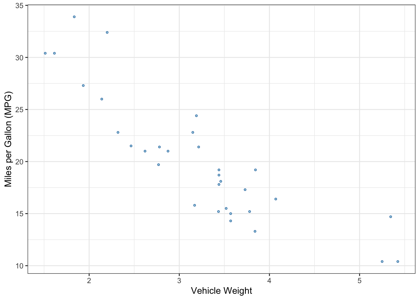
Plotly is a library that allows you to create interactive charts. You can convert static ggplot2 plots into interactive plots using the ggplotly() function.
Below is an example of how to convert a static ggplot2 plot into an interactive Plotly plot:
library(plotly)
Attaching package: 'plotly'The following object is masked from 'package:ggplot2':
last_plotThe following object is masked from 'package:stats':
filterThe following object is masked from 'package:graphics':
layout# Create a ggplot object
p <- ggplot(mtcars, aes(x = wt, y = mpg)) +
geom_point(size = .8, shape = 21, color = "steelblue", fill = "lightblue") + xlab("Vehicle Weight") +
theme_bw()
# Convert the ggplot object to an interactive plot
ggplotly(p)diamonds dataset from the ggplot2 package.# Bar chart of diamond cuts
ggplot(diamonds, aes(x = cut)) +
geom_bar(fill = "skyblue") +
theme_bw()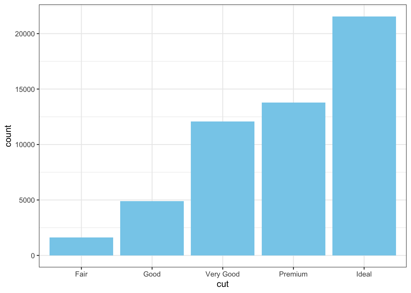
Convert the static bar chart into an interactive chart using Plotly:
# Convert ggplot bar chart to interactive plot
p_bar <- ggplot(diamonds, aes(x = cut)) +
  geom_bar(fill = "skyblue") +
  theme_bw()

ggplotly(p_bar)Try creating a dashboard using the Plotly package, with example data from Plotly and Gapminder data to illustrate interactive charts. Note the use of external fonts from Google Fonts, color choices and animation button and slider control.
# install.packages(c("plotly","tidyverse","RColrBrewer"))
library(plotly)
library(tidyverse)
# Reading in example dataset
df <- read.csv("https://plotly.com/~public.health/17.csv", skipNul = TRUE, encoding = "UTF-8")

# Font management
library(showtext)
font_add_google("EB Garamond","ebgaramond")
t <- list(
  family = "ebgaramond",
  size = 12)

# Create label function for animation button
labels <- function(size, label) {
  list(
    args = c("xbins.size", size),
    label = label,
    method = "restyle"
  )
}

# Create Figure object
fig <- df %>%
  plot_ly(
    x = ~date,
    autobinx = FALSE,
    autobiny = TRUE,
    marker = list(color = "steelblue"),
    name = "date",
    type = "histogram",
    xbins = list(
      end = "2016-12-31 12:00",
      size = "M1",
      start = "1983-12-31 12:00"
    )
  )

# Configure dropdown menu
fig <- fig %>% layout(
  paper_bgcolor = "white",
  plot_bgcolor = "white",
  title = "<b>Shooting Incidents</b><br>use dropdown to change bin size", # HTML to separate line
  xaxis = list(
    type = 'date'
  ),
  yaxis = list(
    title = "Incidents"
  ),
  updatemenus = list(
    list(
      x = 0.1,
      y = 1.15,
      active = 1,
      showactive = TRUE,
      buttons = list(
        labels("D1", "Day"),
        labels("M1", "Month"),
        labels("M6", "Half Year"),
        labels("M12", "Year")
      )
    )
  )
)

fig <- fig %>% layout(font = t) # Add font to text

fig#install.packages("gapminder")
library(gapminder)
library(RColorBrewer)
library(plotly)
# Read in Gapminder data
df <- gapminder
# Font management
t <- list(
family = "corgaramond",
size = 12)
# Create figure object
fig <- df %>%
plot_ly(
x = ~gdpPercap,
y = ~lifeExp,
size = ~pop,
color = ~continent,
colors = c("slateblue3", "steelblue", "firebrick", "forestgreen", "turquoise1"),
# manually select colar
alpha=.5, # translucent glyth
frame = ~year,
text = ~country,
hoverinfo = "text",
type = 'scatter',
mode = 'markers',
fill = ~''
)
# Add font to text
fig <- fig %>% layout(
xaxis = list(
type = "log"
), font = t
)
fig <- fig %>% layout(legend = list(orientation = "h", # show entries horizontally
xanchor = "center", # use center of legend as anchor
x = 0.5, y = 100)) # put legend in center of x-axis
fig <- fig %>% animation_button(
x = 1, xanchor = "right", y = 0, yanchor = "bottom"
)
fig <- fig %>% animation_slider(
currentvalue = list(prefix = "YEAR ", font = list(color="red"))
)
figBy following these examples and exercises, participants will gain practical experience in creating both static and interactive visualizations using R. This session will enhance their ability to communicate data insights effectively through engaging graphics.
ggplot2, demonstrating how to create and customize scatter plots.Plotly to add interactivity to existing ggplot2 plots.Plotly and external fonts.